Numerical Methods for Engineers
7th Edition
ISBN: 9780073397924
Author: Steven C. Chapra Dr., Raymond P. Canale
Publisher: McGraw-Hill Education
bartleby

Videos

Textbook Question
Book Icon
Chapter 24, Problem 46P

The upward velocity of a rocket can be computed by the following formula:

v = u In ( m 0 m 0 q t ) g t

Where v = upword velocity, u = velocity at which fuel is expelled relative to the rocket, m 0 = initial mass of the rocket at time t = 0 ,

q = fuel consumption rate, and g = downword acceleration of gravity ( ( assumed constant = 9 .8 m/s 2 ) . If u = 1800 m/s , m 0 = 160 , 000 kg, and q = 2500 kg/s , use six-segment trapezoidal and Simpson's 1 / 3 rule, six-point Gauss quadrature, and O ( h 8 ) Romberg methods to determine how high the rocket will fly in 30 s. In addition, use numerical differentiation to generate a graph of acceleration as a function of time.

Expert Solution & Answer
Check Mark
To determine

To calculate: The height of the rocket at t=30sec using Six-segment trapezoidal, Simpson’s 1/3 rule, six-point Gauss quadrature and O(h8) Romberg methods. Also, generate a graph of acceleration as a function of time.

Answer to Problem 46P

Solution:

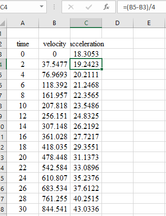
All the results are summarized in the table below,

1 2 3 4
n a 4.0634% 0.04927% 0.01159%
1 12668.115 10896.965 10875.5283 10880.57300
2 11339.7525 10880.8875 10879.31183
4 10995.60375 10879.70575
8 10908.68025

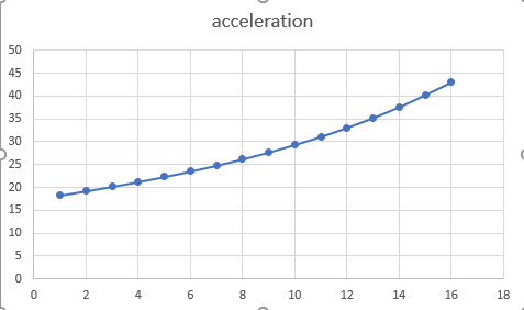
Acceleration graph is shown below.

Numerical Methods for Engineers, Chapter 24, Problem 46P , additional homework tip  1

Explanation of Solution

Given Information:

The formula for the upward velocity of rocket is given as,

v=uln(m0m0qt)gt

Here, v= upward velocity, u=1800 m/s Velocity at which fuel is expelled relative to the rocket

m0=160,000 kg Initial mass of the rocket at time t=a=0, q=2500 kg/s Fuel consumption rate, g=9.8m/s2, Downward acceleration of gravity, b=30 s is the final time.

Formula Used:

6-segment Trapezoidal rule.

I=ba2n[f(a)+2{i=1n1f(a+ih)}+f(b)]

6-segmentSimpson’s 1/3 rule.

I=ba3n[f(x0)+4iodd=1n1f(xi)+2ieven=2n2f(xi)+f(xn)]

Change of variable formula.

t=(b+a)+(ba)td2, dt=(ba)dtd2

Here, a and b are the lower and upper limits of the integral respectively.

Error Calculation.

a=|Actual value-Approx valueActual value|100%

Calculation:

Calculate the upward velocity of the rocket.

v=uln(m0m0qt)gt…… (1)

Substitute thegiven values in equation(1),

v=030(1800ln(160,000160,0002500t)9.8t)dt…… (2)

Apply 6-segment Trapezoidal rule for f(t)=v.

I=ba2n[f(a)+2{i=1n1f(a+ih)}+f(b)]

Here, h=ban

Substitute n=6, a=0 and b=30.

I=3002(6)[f(0)+2{i=15f(0+i(5))}+f(30)]

Expand the above terms.

I=3002(6)[f(0)+2{f(5)+f(10)+f(15)+f(20)+f(25)}+f(30)]…… (3)

Calculate f(0)

f(t)=1800ln(160,000160,0002500t)9.8t

Substitute t=0

f(0)=1800ln(160,000160,000(25000))(9.80)=0

Calculate f(5)

f(t)=1800ln(160,000160,0002500t)9.8t

Substitute t=5

f(5)=1800ln(160,000160,000(25005))(9.85)=97.4222

Calculate f(10)

f(t)=1800ln(160,000160,0002500t)9.8t

Substitute t=10

f(10)=1800ln(160,000160,000(250010))(9.810)=207.818

Similarly, calculate all the function values.

f(15)=333.713,f(20)=478.448f(25)=646.579,f(30)=844.541

Substitute above values in equation(3),

I=302(6)[0+2(97.4222+207.818+333.713+478.448+646.579)+844.541]=10931.2535

The formula for 6-segment Simpson’s 1/3 rule,

I=ba3n[f(x0)+4iodd=1n1f(xi)+2ieven=2n2f(xi)+f(xn)]

Substitute the function values from above,

I=3003(6)[f(0)+4{f(5)+f(15)+f(25)}+2{f(10)+f(20)}+f(30)]=303(6)[0+4{97.4222+333.713+646.579}+2{207.818+478.448}+844.541]=10879.883

The given velocity Integral is,

v=030(1800ln(160,000160,0002500t)9.8t)dt

Change of variable before integrating the function,

t=(b+a)+(ba)td2…… (4)

And

dt=(ba)dtd2…… (5)

Here, a and b are the lower and upper limits of the integral respectively.

Substitute the values of a=0 and b=30 in the equations(4) and (5),

t=15+15tddt=15dtd

Substitute the values of t and dt in equation(2),

v=030(1800ln(160,000160,0002500(15+15td))9.8(15+15td))15dtd

Thus, the transformed function is,

f(td)=(1800ln(160,000160,0002500(15+15td))9.8(15+15td))15

Apply Six-Point Gauss Quadrature formula.

I=0.1713245f(0.932469514)+0.3607616f(0.661209386)+0.4679139f(0.238619186)+0.4679139f(0.238619186)+0.3607616f(0.661209386)+0.1713245f(0.932469514)

Calculate f(0.932469514).

f(td)=(1800ln(160,000160,0002500(15+15td))9.8(15+15td))15

Substitute td=0.932469514.

f(0.932469514)=(1800ln(1600001600002500(15+15(0.932469514)))9.8(15+15(0.932469514)))(15)=281.855

Calculate f(0.661209386).

f(td)=(1800ln(160,000160,0002500(15+15td))9.8(15+15td))15

Substitute td=0.661209386.

f(0.661209386)=(1800ln(1600001600002500(15+15(0.661209386)))9.8(15+15(0.661209386)))(15)=1486.79

Similarly, calculate all function values.

f(0.238619186)=3628.30f(0.238619186)=6527.55f(0.661209386)=9654.10f(0.932469514)=12024.4

Substitute the values in Six-Point Gauss Quadrature formula.

I=0.1713245(281.855)+0.3607616(1486.79)+0.4679139(3628.30)+0.4679139(6527.55)+0.3607616(9654.10)+0.1713245(12024.4)=10879.63166

Apply Romberg Integration.

Choose h=30(distance between two consecutive ordinates), the values of v are,

t 0 30
v x0=0 x1=844.541

Substitute value from above and calculate I(h),

I(h)=h2(x0+x1)=302(0+844.541)=12668.115

Choose h=15, the values of v are,

t 0 15 30
v x0=0 x1=333.713 x2=844.541

Substitute values from above and calculate I(h2),

I(h2)=h2(x0+2x1+x2)=152(0+2(333.713)+844.541)=11339.7525

Choose h=7.5, the values of v are,

t 0 7.5 15 22.5 30
v x0=0 x1=150.856 x2=333.713 x3=559.241 x4=844.541

Substitute values from above and calculate I(h4),

I(h4)=h2(x0+2(x1+x2+x3)+x4)=7.52(0+2(150.856+333.713+559.241)+844.541)=10995.60375

Choose h=3.75, the values of v are,

t 0 3.75 7.5 11.25
v x0=0 x1=71.9349 x2=150.856 x3=237.725
15 18.75 22.5 26.25 30
x4=333.713 x5=440.275 x6=559.241 x7=692.966 x8=844.541

Substitute values from above and calculate I(h8),

I(h8)=h2(x0+2(x1+x2+x3+x4+x5+x6+x7)+x8)=3.752(0+2(71.9349+150.856+237.725+333.713+440.275+559.241+692.966)+844.541)=10908.68025

Substitute values from above and calculate I(h,h2),

I(h,h2)=13[4I(h2)I(h)]=13[4(11339.7525)12668.115]=10896.965

Calculate the approximate error,

a=|Actual value-Approx valueActual value|100%

Substitute values from above.

a=|10896.96511339.752510896.965|100%a=4.0634%

Substitute values from above and calculate I(h2,h4),

I(h2,h4)=13[4I(h4)I(h2)]=13[4(10995.60375)11339.7525]=10880.8875

Substitute values from above and calculate I(h4,h8),

I(h4,h8)=13[4I(h8)I(h4)]=13[4(10908.68025)10995.60375]=10879.70575

Substitute values from above and calculate I(h,h2,h4),

I(h,h2,h4)=13[4I(h2,h4)I(h,h2)]=13[4(10880.8875)10896.965]=10875.5283

Calculate the approximate error,

a=|Actual value-Approx valueActual value|100%

Substitute values from above,

a=|10875.528310880.887510875.5283|100%a=0.04927%

Substitute values from above and calculate I(h2,h4,h8),

I(h2,h4,h8)=13[4I(h4,h8)I(h2,h4)]=13[4(10879.70575)10880.8875]=10879.31183

Substitute values from above and calculate I(h,h2,h4,h8),

I(h,h2,h4,h8)=13[4I(h2,h4,h8)I(h,h2,h4)]=13[4(10879.31183)10875.5283]=10880.5730

Calculate the approximate error as,

a=|Actual value-Approx valueActual value|100%

Substitute values from above.

a=|10880.5730010879.3118310880.57300|100%a=0.01159%

All above calculated results are summarized in the table below,

1 2 3 4
n a 4.0634% 0.04927% 0.01159%
1 12668.115 10896.965 10875.5283 10880.57300
2 11339.7525 10880.8875 10879.31183
4 10995.60375 10879.70575
8 10908.68025

UseNumerical differentiation to calculate acceleration as a function of time.

Apply finite-divided differences for h=2,

a(0)=dv(0)dt=3(76.9693)+4(37.5477)02(2)=18.3053

Apply centred differences to calculate the intermediate values,

a(2)=dv(2)dt=76.969302(2)=19.2423

Similarly, calculate all intermediate values of acceleration.

Apply backward difference for the last value at t = 30 s,

a(30)=dv(30)dt=3(844.5406)+4(761.255)+683.53452(2)=43.0036

All of the results are displayed in the following table and graph,

Numerical Methods for Engineers, Chapter 24, Problem 46P , additional homework tip  2

Select the time and acceleration column and go to insert chart and scattered chart. The graph of acceleration verses time is plotted as follows:

Numerical Methods for Engineers, Chapter 24, Problem 46P , additional homework tip  3

Want to see more full solutions like this?

Subscribe now to access step-by-step solutions to millions of textbook problems written by subject matter experts!
Students have asked these similar questions
When an object is dropped straight down, the distance (in feet) that it travels in t seconds is given by s(t) = - 16t. Find the velocity at each of the following times. a. After 3 seconds. b. After 6 seconds. c. After 8 seconds. d. Find the acceleration. a. The velocity after 3 seconds is ft/sec.
The velocity of a particle along the s-axis is given by v = 659/8 where s is in millimeters and vis in millimeters per second. Determine the acceleration when s is 4.1 millimeters. Answer: a = i eTextbook and Media mm/s²
The upward velocity of a rocket can be computed by the following formula: v = uln mo mo-qt - gt where v= upward velocity, u = the velocity at which fuel is expelled relative to the rocket, mo = the initial mass of the rocket at time t = 0, q = the fuel consumption rate, and g = the downward acceleration of gravity = 9.81 m/s2. If u = 1800 m/s, mo = 160,000 kg, and q = 2600 kg/s, Compute the time at which v= 750 m/s by implementing any efficient bracketing method with initial values of t= 10 and 50 s. Determine your result so that it is within 1% of the true value. (Round the final answer to four decimal places.) The time when v= 750 m/s is t= S.

Chapter 24 Solutions

Numerical Methods for Engineers

Ch. 24 - One of your colleagues has designed a new...Ch. 24 - Video an giography is used to measure blood flow...Ch. 24 - 24.14 Perform the same computation as in Sec....Ch. 24 - Perform the same computation as in Sec. 24.2, but...Ch. 24 - 24.16 As in Sec. 24.2, compute F using the...Ch. 24 - Stream cross-sectional areas (A) are required for...Ch. 24 - 24.18 As described in Prob. 24.17, the...Ch. 24 - 24.21 A transportation engineering study requires...Ch. 24 - 24.22 A wind force distributed against the side of...Ch. 24 - 24.23 Water exerts pressure on the upstream ...Ch. 24 - 24.24 To estimate the size of a new dam, you have...Ch. 24 - The data listed in the following table gives...Ch. 24 - The heat flux q is the quantity of heat flowing...Ch. 24 - 24.27 The horizontal surface area of a lake at a...Ch. 24 - 24.28 Perform the same computation as in Sec....Ch. 24 - 24.29 Repeat Prob. 24.28, but use five...Ch. 24 - Repeat Prob. 24.28, but use Romberg integration to...Ch. 24 - Faradays law characterizes the voltage drop across...Ch. 24 - 24.32 Based on Faraday’s law (Prob. 24.31), use...Ch. 24 - Suppose that the current through a resistor is...Ch. 24 - If a capacitor initially holds no charge, the...Ch. 24 - 24.35 Perform the same computation as in Sec....Ch. 24 - 24.36 Repeat Prob. 24.35, but use (a) Simpson’s ...Ch. 24 - 24.37 Compute work as described in Sec. 24.4, but...Ch. 24 - As was done in Sec. 24.4, determine the work...Ch. 24 - 24.39 The work done on an object is equal to the...Ch. 24 - The rate of cooling of a body (Fig. P24.40) can be...Ch. 24 - 24.41 A rod subject to an axial load (Fig....Ch. 24 - If the velocity distribution of a fluid flowing...Ch. 24 - 24.43 Using the following data, calculate the work...Ch. 24 - 24.44 A jet fighter’s position on an aircraft...Ch. 24 - 24.45 Employ the multiple-application Simpson’s...Ch. 24 - The upward velocity of a rocket can be computed by...Ch. 24 - Referring to the data from Problem 20.61, find the...Ch. 24 - Fully developed flow moving through a 40-cm...Ch. 24 - Fully developed flow of a Bingham plasticfluid...Ch. 24 - 24.50 The enthalpy of a real gas is a ...Ch. 24 - Given the data below, find the isothermal work...Ch. 24 - 24.52 The Rosin-Rammler-Bennet (RRB) equation is...Ch. 24 - For fluid flow over a surface, the heat flux to...Ch. 24 - The pressure gradient for laminar flow through a...Ch. 24 - 24.55 Velocity data for air are collected at...
Knowledge Booster
Background pattern image
Advanced Math
Learn more about
Need a deep-dive on the concept behind this application? Look no further. Learn more about this topic, advanced-math and related others by exploring similar questions and additional content below.
Recommended textbooks for you
Text book image
Algebra & Trigonometry with Analytic Geometry
Algebra
ISBN:9781133382119
Author:Swokowski
Publisher:Cengage
Text book image
Algebra: Structure And Method, Book 1
Algebra
ISBN:9780395977224
Author:Richard G. Brown, Mary P. Dolciani, Robert H. Sorgenfrey, William L. Cole
Publisher:McDougal Littell
Text book image
College Algebra
Algebra
ISBN:9781337282291
Author:Ron Larson
Publisher:Cengage Learning
Text book image
Trigonometry (MindTap Course List)
Trigonometry
ISBN:9781337278461
Author:Ron Larson
Publisher:Cengage Learning
Evaluating Indefinite Integrals; Author: Professor Dave Explains;https://www.youtube.com/watch?v=-xHA2RjVkwY;License: Standard YouTube License, CC-BY
Calculus - Lesson 16 | Indefinite and Definite Integrals | Don't Memorise; Author: Don't Memorise;https://www.youtube.com/watch?v=bMnMzNKL9Ks;License: Standard YouTube License, CC-BY