Videos
Perform ANOVA to test the significance at 1% level of significance.
Answer to Problem 37E
The ANOVA for the given data is shown below:
| Source |
Degrees of freedom |
Sum of squares |
Mean sum of squares | F-ratio |
|
Fabric A | 2 | 4,414.658 | 2207.329 | 2259.293 |
|
Type of exposure B | 1 | 47.255 | 47.255 | 48.36745 |
|
Degree of exposure C | 2 | 983.566 | 491.783 | 503.3603 |
|
Fabric direction D | 1 | 0.044 | 0.044 | 0.045036 |
| Interaction AB | 2 | 30.606 | 15.303 | 15.66325 |
| Interaction AC | 2 | 1,101.754 | 275.446 | 281.9304 |
| Interaction AD | 2 | 0.94 | 0.47 | 0.481064 |
| Interaction BC | 2 | 4.282 | 2.141 | 2.191402 |
| Interaction BD | 1 | 0.273 | 0.273 | 0.279427 |
| Interaction CD | 2 | 0.494 | 0.247 | 0.252815 |
| Interaction ABC | 4 | 14.856 | 3.714 | 3.801433 |
| Interaction ABD | 2 | 8.144 | 4.072 | 4.167861 |
|
Interaction ACD | 4 | 3.068 | 0.767 | 0.785056 |
|
Interaction BCD | 2 | 0.56 | 0.28 | 0.286592 |
| Interaction ABCD | 4 | 1.389 | 0.347 | 0.355 |
| Error | 36 | 35.172 | 0.977 | |
| Total | 71 | 6,647.091 | 9.621 |
There is sufficient of evidence to conclude that there is an effect of fabric on the extent of color change at 1% level of significance.
There is sufficient of evidence to conclude that there is an effect exposure type on the extent of color change at 1% level of significance.
There is sufficient of evidence to conclude that there is an effect of exposure level on the extent of color change at 1% level of significance.
There is no sufficient of evidence to conclude that there is an effect of fabric direction on the extent of color change at 1% level of significance.
There is sufficient of evidence to conclude that there is an interaction effect of fabric and exposure type on the extent of color change at 1% level of significance.
There is sufficient of evidence to conclude that there is an interaction effect of fabric and exposure level on the extent of color change at 1% level of significance.
There is no sufficient of evidence to conclude that there is an interaction effect of fabric and fabric direction on the extent of color change at 1% level of significance.
There is no sufficient of evidence to conclude that there is an interaction effect of exposure type and exposure level on the extent of color change at 1% level of significance.
There is no sufficient of evidence to conclude that there is an interaction effect of exposure type and fabric direction on the extent of color change at 1% level of significance.
There is no sufficient of evidence to conclude that there is an interaction effect of exposure level and fabric direction on the extent of color change at 1% level of significance.
There is no sufficient of evidence to conclude that there is an interaction effect of fabric, exposure type and exposure level on the extent of color change at 1% level of significance.
There is no sufficient of evidence to conclude that there is an interaction effect of fabric, exposure type and fabric direction on the extent of color change at 1% level of significance.
There is no sufficient of evidence to conclude that there is an interaction effect of fabric, exposure level and fabric direction on the extent of color change at 1% level of significance.
There is no sufficient of evidence to conclude that there is an interaction effect of exposure type, exposure level and fabric direction on the extent of color change at 1% level of significance.
There is no sufficient of evidence to conclude that there is an interaction effect of fabric, exposure type, exposure level and fabric direction on the extent of color change at 1% level of significance.
Explanation of Solution
Given info:
An experiment was conducted to test the effect of fabric, type of exposure, level of exposure and fabric direction on the color change of the fabric. Two observation were noted for each of the four factors.
Calculation:
The general ANOVA table is given below:
| Source | Degrees of freedom | Sum of squares | Mean sum of squares | F-ratio |
| Factor A | ||||
| Factor B | ||||
| Factor C | ||||
| Factor D | ||||
| Interaction AB | ||||
| Interaction ABC | ||||
| Error | ||||
| Total |
The sum of squares for each factor and interaction is calculated by multiplying the mean sum of squares with its corresponding degrees of freedom.
Sum of squares excluding ABCD:
| Source | Sum of squares |
| A | 4,414.658 |
| B | 47.255 |
| C | 983.566 |
| D | 0.044 |
| AB | 30.606 |
| AC | 1,101.784 |
| AD | 0.94 |
| BC | 4.282 |
| BD | 0.273 |
| CD | 0.494 |
| ABC | 14.856 |
| ABD | 8.144 |
| ACD | 3.068 |
| BCD | 0.56 |
| Error | 35.172 |
| Total | 6,647.091 |
Using the above table SSABCD can be calculated:
The mean sum of squares for the interaction ABCD is given below:
Thus, the mean sum of squares for the interaction ABCD is 0.347.
The ANOVA for the given data is shown below:
| Source | Degrees of freedom |
Sum of squares |
Mean sum of squares | F-ratio |
|
Fabric A | 4,414.658 | 2207.329 | 2,259.293 | |
|
Type of exposure B | 47.255 | 47.255 | 48.36745 | |
|
Degree of exposure C | 983.566 | 491.783 | 503.3603 | |
|
Fabric direction D | 0.044 | 0.044 | 0.045036 | |
|
Interaction AB | 30.606 | 15.303 | 15.66325 | |
|
Interaction AC | 1,101.754 | 275.446 | 281.9304 | |
|
Interaction AD | 0.94 | 0.47 | 0.481064 | |
|
Interaction BC | 4.282 | 2.141 | 2.191402 | |
|
Interaction BD | 0.273 | 0.273 | 0.279427 | |
|
Interaction CD | 0.494 | 0.247 | 0.252815 | |
|
Interaction ABC | 14.856 | 3.714 | 3.801433 | |
|
Interaction ABD | 8.144 | 4.072 | 4.167861 | |
|
Interaction ACD | 3.068 | 0.767 | 0.785056 | |
|
Interaction BCD | 0.56 | 0.28 | 0.286592 | |
|
Interaction ABCD | 1.389 | 0.347 | 0.355 | |
| Error | 35.172 | 0.977 | ||
| Total | 6,647.091 | 9.621 |
Where,
The F statistic for each factor is obtained by dividing the mean sum of squares with the mean sum of squares due to error.
Testing the main effects:
Testing the Hypothesis for the factor A:
Null hypothesis:
That is, there is no significant difference in the extent of color change due to the three levels of fabrics.
Alternative hypothesis:
That is, there is significant difference in the extent of color change due to the three levels of fabrics.
Testing the Hypothesis for the factor B:
Null hypothesis:
That is, there is no significant difference in the extent of color change due to the two levels of exposure type.
Alternative hypothesis:
That is, there is a significant difference in the extent of color change due to the two levels of exposure type.
Testing the Hypothesis for the factor C:
Null hypothesis:
That is, there is no significant difference in the extent of color change due to the three levels of exposure level.
Alternative hypothesis:
That is, there is a significant difference in the extent of color change due to the three levels of exposure level.
Testing the Hypothesis for the factor D:
Null hypothesis:
That is, there is no significant difference in the extent of color change due to the two levels of fabric direction.
Alternative hypothesis:
That is, there is a significant difference in the extent of color change due to the two levels of fabric direction.
Testing the Hypothesis for the interaction effect of AB:
Null hypothesis:
That is, there is no significant difference in the extent of color change due to the interaction between fabric and exposure type.
Alternative hypothesis:
That is, there is significant difference in the extent of color change due to the interaction between fabric and exposure type.
Testing the Hypothesis for the interaction effect AC:
Null hypothesis:
That is, there is no significant difference in the extent of color change due to the interaction between fabric and exposure level.
Alternative hypothesis:
That is, there is a significant difference in the extent of color change due to the interaction between fabric and exposure level.
Testing the Hypothesis for the interaction effect AD:
Null hypothesis:
That is, there is no significant difference in the extent of color change due to the interaction between fabric and fabric direction.
Alternative hypothesis:
That is, there is a significant difference in the extent of color change due to the interaction between fabric and fabric direction.
Testing the Hypothesis for the interaction effect BC:
Null hypothesis:
That is, there is no significant difference in the extent of color change due to the interaction between exposure type and exposure level.
Alternative hypothesis:
That is, there is significant difference in the extent of color change due to the interaction between exposure type and exposure level.
Testing the Hypothesis for the interaction effect BD:
Null hypothesis:
That is, there is no significant difference in the extent of color change due to the interaction between exposure type and fabric direction.
Alternative hypothesis:
That is, there is significant difference in the extent of color change due to the interaction between exposure type and fabric direction.
Testing the Hypothesis for the interaction effect CD:
Null hypothesis:
That is, there is no significant difference in the extent of color change due to the interaction between exposure level and fabric direction.
Alternative hypothesis:
That is, there is significant difference in the extent of color change due to the interaction between exposure level and fabric direction.
Testing the Hypothesis for the interaction effect ABC:
Null hypothesis:
That is, there is no significant difference in the extent of color change due to the interaction between fabric, exposure type and exposure level.
Alternative hypothesis:
That is, there is a significant difference in the extent of color change due to the interaction between fabric, exposure type and exposure level.
Testing the Hypothesis for the interaction effect ABD:
Null hypothesis:
That is, there is no significant difference in the extent of color change due to the interaction between fabric, exposure type and fabric direction.
Alternative hypothesis:
That is, there is a significant difference in the extent of color change due to the interaction between fabric, exposure type and fabric direction.
Testing the Hypothesis for the interaction effect ACD:
Null hypothesis:
That is, there is no significant difference in the extent of color change due to the interaction between fabric, exposure level and fabric direction.
Alternative hypothesis:
That is, there is a significant difference in the extent of color change due to the interaction between fabric, exposure level and fabric direction.
Testing the Hypothesis for the interaction effect BCD:
Null hypothesis:
That is, there is no significant difference in the extent of color change due to the interaction between exposure type, exposure level and fabric direction.
Alternative hypothesis:
That is, there is a significant difference in the extent of color change due to the interaction between exposure type, exposure level and fabric direction.
Testing the Hypothesis for the interaction effect ABCD:
Null hypothesis:
That is, there is no significant difference in the extent of color change due to the interaction between exposure type, exposure level and fabric direction.
Alternative hypothesis:
That is, there is a significant difference in the extent of color change due to the interaction between fabric, exposure type, exposure level and fabric direction.
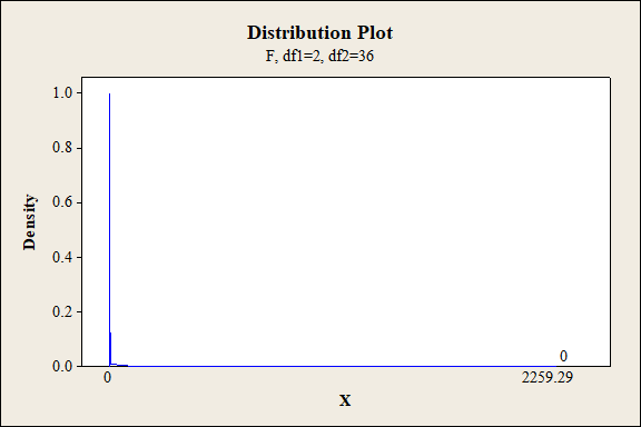
P-value for the main effect of A:
Software procedure:
Step-by-step procedure to find the P-value is given below:
- Click on Graph, select View Probability and click OK.
- Select F, enter 2 in numerator df and 36 in denominator df.
- Under Shaded Area Tab select X value under Define Shaded Area By and select right tails.
- Choose X value as 2,259.29.
- Click OK.
Output obtained from MINITAB is given below:
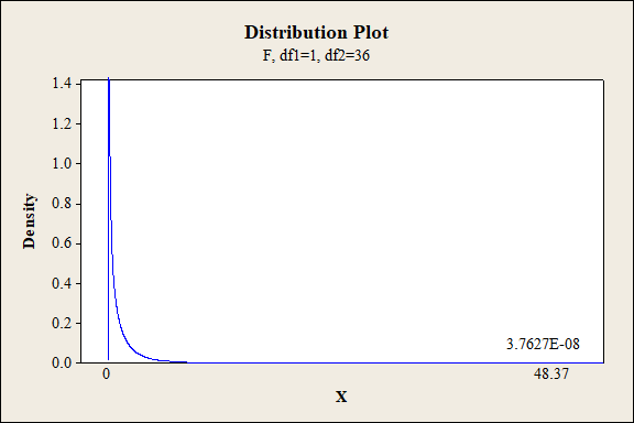
P-value for the main effect of B:
Software procedure:
Step-by-step procedure to find the P-value is given below:
- Click on Graph, select View Probability and click OK.
- Select F, enter 1 in numerator df and 36 in denominator df.
- Under Shaded Area Tab select X value under Define Shaded Area By and select right tails.
- Choose X value as 48.37.
- Click OK.
Output obtained from MINITAB is given below:
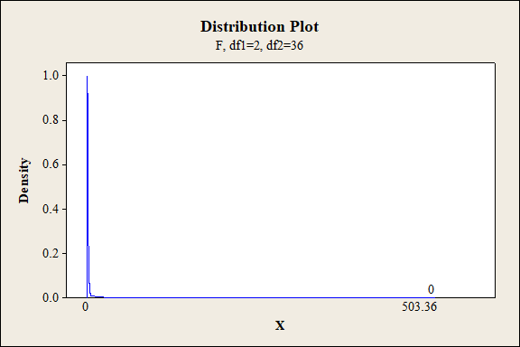
P-value for the main effect of C:
Software procedure:
Step-by-step procedure to find the P-value is given below:
- Click on Graph, select View Probability and click OK.
- Select F, enter 2 in numerator df and 36 in denominator df.
- Under Shaded Area Tab select X value under Define Shaded Area By and select right tails.
- Choose X value as 503.36.
- Click OK.
Output obtained from MINITAB is given below:
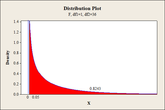
P-value for the main effect of D:
Software procedure:
Step-by-step procedure to find the P-value is given below:
- Click on Graph, select View Probability and click OK.
- Select F, enter 1 in numerator df and 36 in denominator df.
- Under Shaded Area Tab select X value under Define Shaded Area By and select right tails.
- Choose X value as 0.05.
- Click OK.
Output obtained from MINITAB is given below:
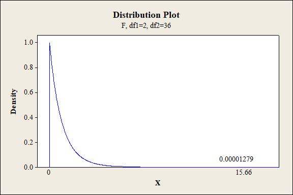
P-value for the interaction effect of A and B:
Software procedure:
Step-by-step procedure to find the P-value is given below:
- Click on Graph, select View Probability and click OK.
- Select F, enter 2 in numerator df and 36 in denominator df.
- Under Shaded Area Tab select X value under Define Shaded Area By and select right tails.
- Choose X value as 15.66.
- Click OK.
Output obtained from MINITAB is given below:
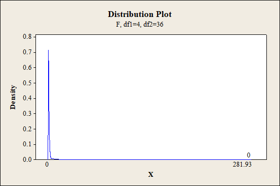
P-value for the interaction effect of A and C:
Software procedure:
Step-by-step procedure to find the P-value is given below:
- Click on Graph, select View Probability and click OK.
- Select F, enter 4 in numerator df and 36 in denominator df.
- Under Shaded Area Tab select X value under Define Shaded Area By and select right tails.
- Choose X value as 281.93.
- Click OK.
Output obtained from MINITAB is given below:
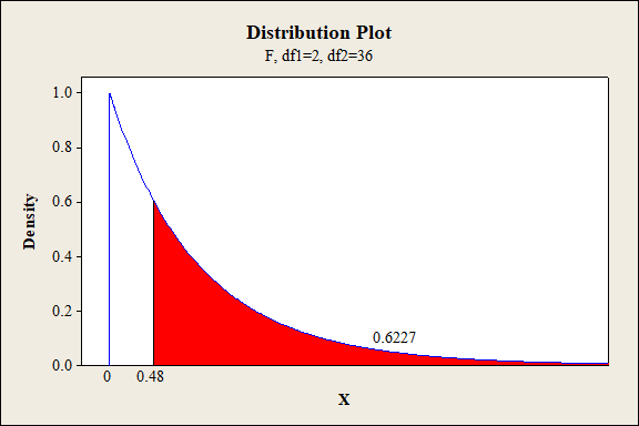
P-value for the interaction effect of A and D:
Software procedure:
Step-by-step procedure to find the P-value is given below:
- Click on Graph, select View Probability and click OK.
- Select F, enter 2 in numerator df and 36 in denominator df.
- Under Shaded Area Tab select X value under Define Shaded Area By and select right tails.
- Choose X value as 0.48.
- Click OK.
Output obtained from MINITAB is given below:
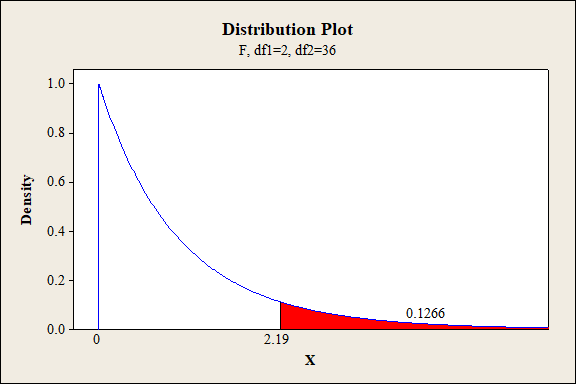
P-value for the interaction effect of B and C:
Software procedure:
Step-by-step procedure to find the P-value is given below:
- Click on Graph, select View Probability and click OK.
- Select F, enter 2 in numerator df and 36 in denominator df.
- Under Shaded Area Tab select X value under Define Shaded Area By and select right tails.
- Choose X value as 2.19.
- Click OK.
Output obtained from MINITAB is given below:
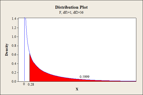
P-value for the interaction effect of B and D:
Software procedure:
Step-by-step procedure to find the P-value is given below:
- Click on Graph, select View Probability and click OK.
- Select F, enter 1 in numerator df and 36 in denominator df.
- Under Shaded Area Tab select X value under Define Shaded Area By and select right tails.
- Choose X value as 0.28.
- Click OK.
Output obtained from MINITAB is given below:
P-value for the interaction effect of C and D:
Software procedure:
Step-by-step procedure to find the P-value is given below:
- Click on Graph, select View Probability and click OK.
- Select F, enter 2 in numerator df and 36 in denominator df.
- Under Shaded Area Tab select X value under Define Shaded Area By and select right tails.
- Choose X value as 0.25.
- Click OK.
Output obtained from MINITAB is given below:

P-value for the interaction effect of A, B and C:
Software procedure:
Step-by-step procedure to find the P-value is given below:
- Click on Graph, select View Probability and click OK.
- Select F, enter 4 in numerator df and 36 in denominator df.
- Under Shaded Area Tab select X value under Define Shaded Area By and select right tails.
- Choose X value as 3.80.
- Click OK.
Output obtained from MINITAB is given below:
P-value for the interaction effect of A, B and D:
Software procedure:
Step-by-step procedure to find the P-value is given below:
- Click on Graph, select View Probability and click OK.
- Select F, enter 2 in numerator df and 36 in denominator df.
- Under Shaded Area Tab select X value under Define Shaded Area By and select right tails.
- Choose X value as 4.17.
- Click OK.
Output obtained from MINITAB is given below:
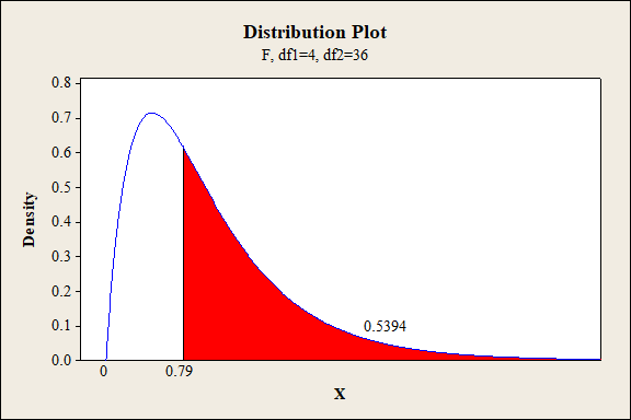
P-value for the interaction effect of A, C and D:
Software procedure:
Step-by-step procedure to find the P-value is given below:
- Click on Graph, select View Probability and click OK.
- Select F, enter 4 in numerator df and 36 in denominator df.
- Under Shaded Area Tab select X value under Define Shaded Area By and select right tails.
- Choose X value as 0.79.
- Click OK.
Output obtained from MINITAB is given below:
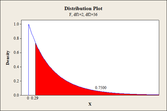
P-value for the interaction effect of B, C and D:
Software procedure:
Step-by-step procedure to find the P-value is given below:
- Click on Graph, select View Probability and click OK.
- Select F, enter 2 in numerator df and 36 in denominator df.
- Under Shaded Area Tab select X value under Define Shaded Area By and select right tails.
- Choose X value as 0.29.
- Click OK.
Output obtained from MINITAB is given below:
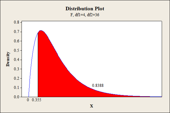
P-value for the interaction effect of A, B, C and D:
Software procedure:
Step-by-step procedure to find the P-value is given below:
- Click on Graph, select View Probability and click OK.
- Select F, enter 4 in numerator df and 36 in denominator df.
- Under Shaded Area Tab select X value under Define Shaded Area By and select right tails.
- Choose X value as 0.355.
- Click OK.
Output obtained from MINITAB is given below:
Conclusion:
For the main effect of A:
The P- value for the factor A (fabric) is 0.000 and the level of significance is 0.01.
Here, the P- value is lesser than the level of significance.
That is,
Thus, the null hypothesis is rejected,
Hence, there is sufficient of evidence to conclude that there is an effect of fabric on the extent of color change at 1% level of significance.
For main effect of B:
The P- value for the factor B (exposure level) is 0.000 and the level of significance is 0.01.
Here, the P- value is lesser than the level of significance.
That is,
Thus, the null hypothesis is not rejected.
Hence, there is sufficient of evidence to conclude that there is an effect exposure type on the extent of color change at 1% level of significance.
For main effect of C:
The P- value for the factor C (exposure level) is 0.000 and the level of significance is 0.01.
Here, the P- value is lesser than the level of significance.
That is,
Thus, the null hypothesis is rejected.
Hence, there is sufficient of evidence to conclude that there is an effect of exposure level on the extent of color change at 1% level of significance.
For main effect of D:
The P- value for the factor D (fabric direction) is 0.8243 and the level of significance is 0.01.
Here, the P- value is greater than the level of significance.
That is,
Thus, the null hypothesis is not rejected.
Hence, there is no sufficient of evidence to conclude that there is an effect of fabric direction on the extent of color change at 1% level of significance.
Interaction effect of factor A and B:
The P- value for the interaction effect AB (fabric and exposure type) is 0.000 and the level of significance is 0.01.
Here, the P- value is lesser than the level of significance.
That is,
Thus, the null hypothesis is rejected,
Hence, there is sufficient of evidence to conclude that there is an interaction effect of fabric and exposure type on the extent of color change at 1% level of significance.
Interaction effect of factor A and C:
The P- value for the interaction effect AC (fabric and exposure level) is 0.000 and the level of significance is 0.01.
Here, the P- value is lesser than the level of significance.
That is,
Thus, the null hypothesis is rejected.
Hence, there is sufficient of evidence to conclude that there is an interaction effect of fabric and exposure level on the extent of color change at 1% level of significance.
Interaction effect of factor A and D:
The P- value for the interaction effect AD (fabric and fabric direction) is 0.6227 and the level of significance is 0.01.
Here, the P- value is greater than the level of significance.
That is,
Thus, the null hypothesis is not rejected.
Hence, there is no sufficient of evidence to conclude that there is an interaction effect of fabric and fabric direction on the extent of color change at 1% level of significance.
Interaction effect of factor B and C:
The P- value for the interaction effect BC (exposure type and exposure level) is 0.1266 and the level of significance is 0.01.
Here, the P- value is greater than the level of significance.
That is,
Thus, the null hypothesis is not rejected,
Hence, there is no sufficient of evidence to conclude that there is an interaction effect of exposure type and exposure level on the extent of color change at 1% level of significance.
Interaction effect of factor B and D:
The P- value for the interaction effect BD (exposure type and fabric direction) is 0.5999 and the level of significance is 0.01.
Here, the P- value is greater than the level of significance.
That is,
Thus, the null hypothesis is not rejected,
Hence, there is no sufficient of evidence to conclude that there is an interaction effect of exposure type and fabric direction on the extent of color change at 1% level of significance.
Interaction effect of factor C and D:
The P- value for the interaction effect CD (exposure level and fabric direction) is 0.7801 and the level of significance is 0.01.
Here, the P- value is greater than the level of significance.
That is,
Thus, the null hypothesis is not rejected,
Hence, there is no sufficient of evidence to conclude that there is an interaction effect of exposure level and fabric direction on the extent of color change at 1% level of significance.
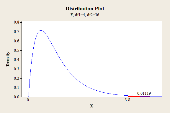
Interaction effect of factor A,B and C:
The P- value for the interaction effect ABC (fabric, exposure type and exposure level) is 0.01119 and the level of significance is 0.01.
Here, the P- value is greater than the level of significance.
That is,
Thus, the null hypothesis is not rejected.
Hence, there is no sufficient of evidence to conclude that there is an interaction effect of fabric, exposure type and exposure level on the extent of color change at 1% level of significance.
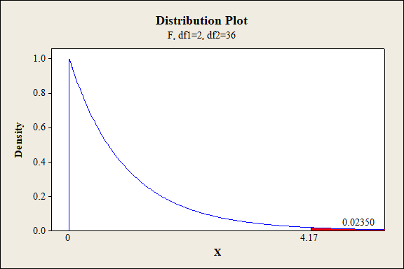
Interaction effect of factor A,B and D:
The P- value for the interaction effect ABD (fabric, exposure type and fabric direction) is 0.0235 and the level of significance is 0.01.
Here, the P- value is greater than the level of significance.
That is,
Thus, the null hypothesis is not rejected.
Hence, there is no sufficient of evidence to conclude that there is an interaction effect of fabric, exposure type and fabric direction on the extent of color change at 1% level of significance.
Interaction effect of factor A,C and D:
The P- value for the interaction effect ACD (fabric, exposure level and fabric direction) is 0.5394 and the level of significance is 0.01.
Here, the P- value is greater than the level of significance.
That is,
Thus, the null hypothesis is not rejected.
Hence, there is no sufficient of evidence to conclude that there is an interaction effect of fabric, exposure level and fabric direction on the extent of color change at 1% level of significance.
Interaction effect of factor B, C and D:
The P- value for the interaction effect BCD (exposure type, exposure level and fabric direction) is 0.7500 and the level of significance is 0.01.
Here, the P- value is greater than the level of significance.
That is,
Thus, the null hypothesis is not rejected.
Hence, there is no sufficient of evidence to conclude that there is an interaction effect of exposure type, exposure level and fabric direction on the extent of color change at 1% level of significance.
Interaction effect of factor A, B, C and D:
The P- value for the interaction effect ABCD (fabric, exposure type, exposure level and fabric direction) is 0.8388 and the level of significance is 0.01.
Here, the P- value is greater than the level of significance.
That is,
Thus, the null hypothesis is not rejected.
Hence, there is no sufficient of evidence to conclude that there is an interaction effect of fabric, exposure type, exposure level and fabric direction on the extent of color change at 1% level of significance.
Therefore, there is significant difference in the extent of color change with respect to the main effect A, B, D and interaction effects AB, AC are significant at 1% level of significance. The remaining second order interactions and third order interaction are not significant at 1% level of significance.
Want to see more full solutions like this?
Chapter 11 Solutions
Bundle: Probability and Statistics for Engineering and the Sciences, 9th + WebAssign Printed Access Card for Devore's Probability and Statistics for ... and the Sciences, 9th Edition, Single-Term


- Find the correlation coefficient between the “modules studied in the last semester and number of hours spend on reading the books” from your collected data.arrow_forwardAortic stenosis refers to a narrowing of the aortic valvein the heart. The article “Correlation Analysis ofStenotic Aortic Valve Flow Patterns Using PhaseContrast MRI” (Annals of Biomed. Engr., 2005:878–887) gave the following data on aortic root diameter(cm) and gender for a sample of patients having variousdegrees of aortic stenosis:M: 3.7 3.4 3.7 4.0 3.9 3.8 3.4 3.6 3.1 4.0 3.4 3.8 3.5F: 3.8 2.6 3.2 3.0 4.3 3.5 3.1 3.1 3.2 3.0a. Compare and contrast the diameter observations forthe two genders.b. Calculate a 10% trimmed mean for each of the twosamples, and compare to other measures of center(for the male sample, the interpolation method mentionedin Section 1.3 must be used).arrow_forwardA medical student at a community college in city Q wants to study the factors affecting the systolic blood pressure of a person (Y). Generally, the systolic blood pressure depends on the BMI of a person (B) and the age of the person A. She wants to test whether or not the BMI has a significant effect on the systolic blood pressure, keeping the age of the person constant. For her study, she collects a random sample of 150 patients from the city and estimates the following regression function: Y= 15.50 +0.90B + 1.10A. (0.48) (0.35) The test statistic of the study the student wants to conduct (Ho: B, =0 vs. H4: B, #0), keeping other variables constant is. (Round your answer to two decimal places.) At the 5% significance level, the student will v the null hypothesis. Keeping BMI constant, she now wants test whether the age of a person (A) has no significant effect or a positive effect on the person's systolic blood pressure. So, the test statistic associated with the one-sided test the…arrow_forward
- Body Fat. In the paper “Total Body Composition by Dual- Photon (153 Gd) Absorptiometry” (American Journal of Clinical Nutrition, Vol. 40, pp. 834–839), R. Mazess et al. studied methods for quantifying body composition. Eighteen randomly selected adults were measured for percentage of body fat, using dual-photon absorptiometry. Each adult’s age and percentage of body fat are shown on the WeissStats site. a. Decide whether you can reasonably apply the regression t-test. If so, then also do part (b). b. Decide, at the 5% significance level, whether the data provide sufficient evidence to conclude that the predictor variable is useful for predicting the response variable.arrow_forwardBody Fat. In the paper “Total Body Composition by Dual- Photon (153 Gd) Absorptiometry” (American Journal of Clinical Nutrition, Vol. 40, pp. 834–839), R. Mazess et al. studied methods for quantifying body composition. Eighteen randomly selected adults were measured for percentage of body fat, using dual-photon absorptiometry. Each adult’s age and percentage of body fat are shown on the WeissStats site. a. Decide whether finding a regression line for the data is reasonable. If so, then also do parts (b)–(d). b. Obtain the coefficient of determination. c. Determine the percentage of variation in the observed values of the response variable explained by the regression, and interpret your answer. d. State how useful the regression equation appears to be for making predictions.arrow_forwardRange of ankle motion is a contributing factor to falls among the elderly. Suppose a team of researchers is studying how combining compression bandages or compression hosiery with different types of footwear affects range of ankle motion. They suspect that more than half of all adults wearing compression bandages and no shoes will see a decrease in range of ankle motion of at least 2° compared to when they are not wearing compression bandages or compression hosiery and are barefoot. They collect sample data from a random sample of 29 adults and determine that 17 see such a decrease in range of ankle motion. They compute a sample proportion of 17 0.586 29 The researchers conduct a one-sample z-test for a proportion, testing Ho : p = 0.500 against H1 :p > 0.500, where p is the proportion of adults whose range of angle motion decreases at least 2° while wearing compression bandages with no shoes. The lower limit of a 95% confidence interval for p is 0.436. Based on this interval, what…arrow_forward
- Expression levels of GeneA and GeneB were measured in 10 cell lines. The researcher would like to know if expression levels of GeneA and GeneB are related.a. Use a parametric method to test if GeneA and GeneB are correlated.b. Use a non-parametric method to test if GeneA and GeneB are correlated.arrow_forwardA study is conducted to determine the relationship between study hours and exam scores, what is the dependent variable in this scenario?arrow_forwardThe linear correlation coefficient for the second data set is R=arrow_forward
- The authors of a paper studied the relationship between y = arch height and scores on a number of different motor ability tests for 218 children. They reported the following correlation coefficients. Motor Ability Test Height of Counter Movement Jump Hopping: Average Height Hopping: Average Power Balance, Closed Eyes, One Leg Toe Flexion Correlation between Test Score and Arch Height -0.10 -0.06 -0.03 0.05 0.04 (a) Identify the value of the correlation coefficient between average hopping height and arch height. r = Interpret the value of the correlation coefficient. O There is a weak negative linear relationship between average hopping height and arch height. O There is a strong positive linear relation average hopping height and arch height. O There is a weak positive linear relationship between average hopping height and arch height. O There is no linear relationship between average hopping height and arch height. O There is a strong negative linear relationship between average…arrow_forwardIn an experiment to determine the impacts of domestic and industrial waste accumulation on plant growth and development, a student took monthly measurements of the height and other growth parameters of maize plants grown in two different types of soil: Soil A (obtained from a domestic and industrial waste dump site) and Soil B (obtained from the University Farms, Legon). A summary of the height data obtained for two-month old maize plants is given below. Soil A Soil B Mean height of maize plants (cm) 39.2 32.6 Standardarrow_forwardA manufacturer ran an experiment to compare the wearing qualities of two different types of automobile tires, A and B. In the experiment, a tire of Type A and one of the type B were randomly assigned and mounted on the rear wheels of each of five cars. the cars were then operated for x miles and the amount of tire wear was recorded (higher number represents more wear). Is there sufficient evidence to conclude that there is a difference in the average wear? Use 0.05 level of significance. Tire A 10.6 9.8 12.3 9.7 8.8 Tire B 10.2 9.4 11.8 9.1 8.3arrow_forward
 Big Ideas Math A Bridge To Success Algebra 1: Stu...AlgebraISBN:9781680331141Author:HOUGHTON MIFFLIN HARCOURTPublisher:Houghton Mifflin Harcourt