
Videos
The accompanying data resulted from an experiment to investigate whether yield from a certain chemical process depended either on the formulation of a particular input or on mixer speed.
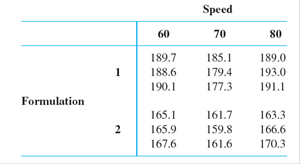
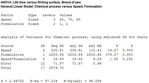
A statistical computer package gave SS(Form) = 2253.44, SS(Speed) = 230.81, SS(Form*Speed) = 18.58, and SSE = 71.87.
a. Does there appear to be interaction between the factors?
b. Does yield appear to depend on either formulation or speed?
c. Calculate estimates of the main effects.
d. The fitted values are
e. Construct a normal probability plot from the residuals given in part (d). Do the ϵijk’s appear to be
a.
Identify whether there is a significant effect from interaction between speed and formulation.
Answer to Problem 18E
There is no sufficient evidence to conclude that there is an effect of interaction between mix speed and formulation on the chemical process.
Explanation of Solution
Given info:
An experiment was carried out to test the effect of formulation and speed on the chemical press. The formulation has two levels and speed has three levels.
The sum of squares due to formulation is 2,253.44, sum of squares due to speed is 230.81, sum of squares due to error is 71.87, sum of squares due to interaction between formulation and speed is 18.58.
Calculation:
Testing the Hypothesis:
Null hypothesis:
That is, the interaction effect between mix speed and formulation has no significant effect on chemical process.
Alternative hypothesis:
That is, the interaction effect between mix speed and formulation has no significant effect on chemical process.
Test statistic:
Software procedure:
Step by step procedure to find the test statistic using Minitab is given below:
- Choose Stat > ANOVA > General Linear Model.
- In Responses, enter the column of Chemical process.
- In Model, enter the column of Speed, Formulation, Speed*Formulation.
- In Results, choose “Analysis of variance table”.
- Click OK in all dialog boxes.
Output obtained from MINITAB is given below:
Conclusion:
Interaction effect of AB:
The P- value for the interaction effect AB is 0.252 and the level of significance is 0.01.
The P- value is lesser than the level of significance.
That is,
Thus, the null hypothesis is not rejected,
Hence, there is no sufficient evidence to conclude that there is an effect of interaction between mix speed and formulation on the chemical process.
b.
Identify whether the yield of the chemical process depends on speed or formulation.
Answer to Problem 18E
The yield of a chemical process depends on both speed and formulation.
Explanation of Solution
From the MINITAB output obtained in part (a), the following can be observed.
For Main effect of factor A speed:
The P- value for the factor A (speed) is 0.000 and the level of significance is 0.01.
The P- value is lesser than the level of significance.
That is,.
Thus, the null hypothesis is rejected,
Hence, there is sufficient evidence to conclude that there is an effect of speed on the yield of chemical process.
For Main effect of factor B formulation:
The P- value for the factor B (formulation) is 0.000 and the level of significance is 0.01.
The P- value is lesser than the level of significance.
That is,
Thus, the null hypothesis is rejected,
Hence, there is sufficient evidence to conclude that there is an effect of formulation on the yield of chemical process.
c.
Find the estimates for the main effects.
Explanation of Solution
Calculation:
Where,
Overall mean effect:
Mean due to the first level of factor A:
Mean due to the second level of factor A:
Main effect of factor A:
At first level:
At second level:
Mean due to the first level of factor B:
Mean due to the second level of factor B:
Mean due to the third level of factor B
Main effect of factor B:
d.
Verify whether the calculated residuals are equal to the given residual values.
Explanation of Solution
Calculation:
The interaction effect for the first level of factor A and the first level of factor B
The interaction effect for the first level of factor A and the second level of factor B
The interaction effect for the first level of factor A and the third level of factor B
Similarly, the remaining values are given below:
| S. No | Values |
| 1 | |
| 2 | |
| 3 | |
| 4 | |
| 5 | |
| 6 |
The fitted values are calculated by using the formula:
Where,
i represents the levels of factor A.
j represents the levels of factor B.
k represents the observation.
The predicted value when
Similarly, the other fitted values are calculated, the table shows the fitted values:
| S. No | 1 | 2 | 3 | 4 | 5 | 6 | 7 | 8 | 9 |
| Fitted values | 189.47 | 189.47 | 189.47 | 166.20 | 166.20 | 166.20 | 180.60 | 180.60 | 180.60 |
| S. No | 10 | 11 | 12 | 13 | 14 | 15 | 16 | 17 | 18 |
| Fitted values | 161.03 | 161.03 | 161.03 | 191.03 | 191.03 | 191.03 | 166.73 | 166.73 | 166.73 |
The residuals values are calculated by using the formula:
The table shows below gives the residuals for each observation:
| S. No |
Observed |
Fitted values | |
| 1 | 189.7 | 189.47 | 0.23 |
| 2 | 188.6 | 189.47 | –0.87 |
| 3 | 190.1 | 189.47 | 0.63 |
| 4 | 165.1 | 166.20 | –1.1 |
| 5 | 165.9 | 166.20 | –0.3 |
| 6 | 167.6 | 166.20 | 1.4 |
| 7 | 185.1 | 180.60 | 4.5 |
| 8 | 179.4 | 180.60 | –1.2 |
| 9 | 177.3 | 180.60 | –3.3 |
| 10 | 161.7 | 161.03 | 0.67 |
| 11 | 159.8 | 161.03 | –1.23 |
| 12 | 161.6 | 161.03 | 0.57 |
| 13 | 189 | 191.03 | –2.03 |
| 14 | 193 | 191.03 | 1.97 |
| 15 | 191.1 | 191.03 | 0.07 |
| 16 | 163.3 | 166.73 | –3.43 |
| 17 | 166.6 | 166.73 | –0.13 |
| 18 | 170.3 | 166.73 | 3.57 |
Hence, the calculated residuals values are equal to given residual values.
e.
Construct a normal probability plot for the residuals obtained in part (d).
Identify whether the residuals are normally distributed.
Answer to Problem 18E
The normal probability of residuals is given below:
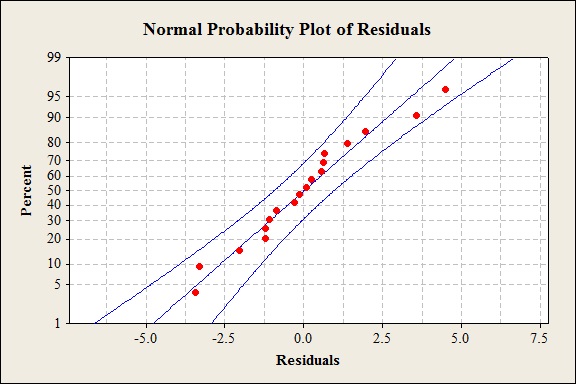
The residuals are normally distributed.
Explanation of Solution
Calculation:
Normal probability plot of residuals:
Software procedure:
Step-by-step procedure to construct a normal probability plot of residuals is given below:
- Click on Graph>Probability plot>Single.
- Click OK.
- Under Graph variables, select the column containing the residual values.
- Click on Distribution and selection Normal.
- Click OK.
Interpretation:
The normal probability plot of residuals suggests that the residuals are normally distributed because the residuals fall approximately on a straight line.
Want to see more full solutions like this?
Chapter 11 Solutions
WEBASSIGN ACCESS FOR PROBABILITY & STATS


- Find the equation of the regression line for the following data set. x 1 2 3 y 0 3 4arrow_forwardUrban Travel Times Population of cities and driving times are related, as shown in the accompanying table, which shows the 1960 population N, in thousands, for several cities, together with the average time T, in minutes, sent by residents driving to work. City Population N Driving time T Los Angeles 6489 16.8 Pittsburgh 1804 12.6 Washington 1808 14.3 Hutchinson 38 6.1 Nashville 347 10.8 Tallahassee 48 7.3 An analysis of these data, along with data from 17 other cities in the United States and Canada, led to a power model of average driving time as a function of population. a Construct a power model of driving time in minutes as a function of population measured in thousands b Is average driving time in Pittsburgh more or less than would be expected from its population? c If you wish to move to a smaller city to reduce your average driving time to work by 25, how much smaller should the city be?arrow_forward
 Calculus For The Life SciencesCalculusISBN:9780321964038Author:GREENWELL, Raymond N., RITCHEY, Nathan P., Lial, Margaret L.Publisher:Pearson Addison Wesley,
 Glencoe Algebra 1, Student Edition, 9780079039897...AlgebraISBN:9780079039897Author:CarterPublisher:McGraw Hill
 Functions and Change: A Modeling Approach to Coll...AlgebraISBN:9781337111348Author:Bruce Crauder, Benny Evans, Alan NoellPublisher:Cengage Learning
 Big Ideas Math A Bridge To Success Algebra 1: Stu...AlgebraISBN:9781680331141Author:HOUGHTON MIFFLIN HARCOURTPublisher:Houghton Mifflin Harcourt