Essentials of Statistics (6th Edition)
6th Edition
ISBN: 9780134685779
Author: Mario F. Triola
Publisher: PEARSON
expand_more
expand_more
format_list_bulleted
Concept explainers
Videos
Textbook Question
Chapter 10.2, Problem 18BSC
Regression and Predictions. Exercises 13–28 use the same data sets as Exercises 13–28 in Section 10-1. In each case, find the regression equation, letting the first variable be the predictor (x) variable, hind the indicated predicted value by following the prediction procedure summarized in Figure 10-5 on page 493.
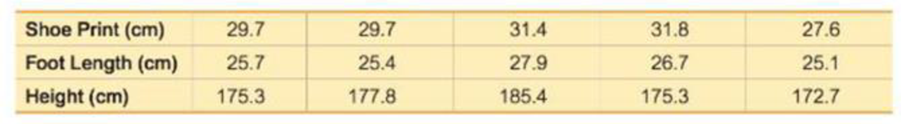
18. CSI Statistics Use the foot lengths and heights to find the best predicted height of a male who has a foot length of 28 cm. Would the result be helpful to police crime scene investigators in trying to describe the male?
Expert Solution & Answer
Want to see the full answer?
Check out a sample textbook solution
Students have asked these similar questions
Regression and Predictions. Exercises 13–28 use the same data sets as Exercises 13–28 in Section 10-1. In each case, find the regression equation, letting the first variable be the predictor (x) variable. Find the indicated predicted value by following the prediction procedure summarized in Figure 10-5 on page 493.
Internet and Nobel Laureates Find the best predicted Nobel Laureate rate for Japan, which has 79.1 Internet users per 100 people. How does it compare to Japan’s Nobel Laureate rate of 1.5 per 10 million people?
Regression and Predictions. Exercises 13–28 use the same data sets as Exercises 13–28 in Section 10-1. In each case, find the regression equation, letting the first variable be the predictor (x) variable. Find the indicated predicted value by following the prediction procedure summarized in Figure 10-5 on page 493.
Manatees Use the listed boat/manatee data. In a year not included in the data below, there were 970,000 registered pleasure boats in Florida. Find the best predicted number of manatee fatalities resulting from encounters with boats. Is the result reasonably close to 79, which was the actual number of manatee fatalities?
Q. Table provided gives data on gross domestic product (GDP) for the United States for the years 1959–2005.
a. Plot the GDP data in current and constant (i.e., 2000) dollars against time.
b. Letting Y denote GDP and X time (measured chronologically starting with 1 for 1959, 2 for 1960, through 47 for 2005), see if the following model fits the GDP data:
Yt = β1 + β2 Xt + ut
Estimate this model for both current and constant-dollar GDP.
c. How would you interpret β2?
d. If there is a difference between β2 estimated for current-dollar GDP and that estimated for constant-dollar GDP, what explains the difference?
e. From your results what can you say about the nature of inflation in the United States over the sample period?
Chapter 10 Solutions
Essentials of Statistics (6th Edition)
Ch. 10.1 - Notation Twenty different statistics students are...Ch. 10.1 - Interpreting r For the some two variables...Ch. 10.1 - Global Warming If we find that there is a linear...Ch. 10.1 - Scatterplots Match these values of r with the five...Ch. 10.1 - Bear Weight and Chest Size Fifty-four wild bears...Ch. 10.1 - Casino Size and Revenue The New York Times...Ch. 10.1 - Garbage Data Set 31 Garbage Weight in Appendix B...Ch. 10.1 - Cereal Killers The amounts of sugar (grams of...Ch. 10.1 - Explore! Exercises 9 and 10 provide two data sets...Ch. 10.1 - Explore! Exercises 9 and 10 provide two data sets...
Ch. 10.1 - Outlier Refer to the accompanying...Ch. 10.1 - Clusters Refer to the following Minitab-generated...Ch. 10.1 - Testing for a Linear Correlation. In Exercises...Ch. 10.1 - Testing for a Linear Correlation. In Exercises...Ch. 10.1 - Testing for a Linear Correlation. In Exercises...Ch. 10.1 - Testing for a Linear Correlation. In Exercises...Ch. 10.1 - Testing for a Linear Correlation. In Exercises...Ch. 10.1 - Testing for a Linear Correlation. In Exercises...Ch. 10.1 - Testing for a Linear Correlation. In Exercises...Ch. 10.1 - Testing for a Linear Correlation. In Exercises...Ch. 10.1 - Testing for a Linear Correlation. In Exercises...Ch. 10.1 - Testing for a Linear Correlation. In Exercises...Ch. 10.1 - Testing for a Linear Correlation. In Exercises...Ch. 10.1 - Testing for a Linear Correlation. In Exercises...Ch. 10.1 - Testing for a Linear Correlation. In Exercises...Ch. 10.1 - Testing for a Linear Correlation. In Exercises...Ch. 10.1 - Testing for a Linear Correlation. In Exercises...Ch. 10.1 - Testing for a Linear Correlation. In Exercises...Ch. 10.1 - Transformed Data In addition to testing for a...Ch. 10.1 - Finding Critical r Values Table A-6 lists critical...Ch. 10.2 - Notation Different hotels on Las Vegas Boulevard...Ch. 10.2 - Notation What is the difference between the...Ch. 10.2 - Best-Fit Line a. What is a residual? b. In what...Ch. 10.2 - Correlation and Slope What is the relationship...Ch. 10.2 - Making Predictions. In Exercises 58, let the...Ch. 10.2 - Making Predictions. In Exercises 58, let the...Ch. 10.2 - Making Predictions. In Exercises 58, let the...Ch. 10.2 - Making Predictions. In Exercises 58, let the...Ch. 10.2 - Finding the Equation of the Regression Line. In...Ch. 10.2 - Finding the Equation of the Regression Line. In...Ch. 10.2 - Effects of an Outlier Refer to the Mini...Ch. 10.2 - Effects of Clusters Refer to the Minitab-generated...Ch. 10.2 - Regression and Predictions. Exercises 1328 use the...Ch. 10.2 - Regression and Predictions. Exercises 1328 use the...Ch. 10.2 - Regression and Predictions. Exercises 1328 use the...Ch. 10.2 - Regression and Predictions. Exercises 1328 use the...Ch. 10.2 - Regression and Predictions. Exercises 1328 use the...Ch. 10.2 - Regression and Predictions. Exercises 1328 use the...Ch. 10.2 - Regression and Predictions. Exercises 1328 use the...Ch. 10.2 - Regression and Predictions. Exercises 1328 use the...Ch. 10.2 - Regression and Predictions. Exercises 1328 use the...Ch. 10.2 - Regression and Predictions. Exercises 1328 use the...Ch. 10.2 - Regression and Predictions. Exercises 1328 use the...Ch. 10.2 - Regression and Predictions. Exercises 1328 use the...Ch. 10.2 - Regression and Predictions. Exercises 13-28 use...Ch. 10.2 - Regression and Predictions. Exercises 13-28 use...Ch. 10.2 - Regression and Predictions. Exercises 13-28 use...Ch. 10.2 - Regression and Predictions. Exercises 13-28 use...Ch. 10.2 - Least-Squares Property According to the...Ch. 10.3 - Regression If the methods of this section are used...Ch. 10.3 - Level of Measurement Which of the levels of...Ch. 10.3 - Notation What do r, rs , and ps denote? Why is the...Ch. 10.3 -
4. Efficiency The efficiency of the rank...Ch. 10.3 - In Exercises 5 and 6, use the scatterplot to find...Ch. 10.3 - In Exercises 5 and 6, use the scatterplot to find...Ch. 10.3 - Testing for Rank Correlation. In Exercises 712,...Ch. 10.3 - Prob. 8BSCCh. 10.3 - Testing for Rank Correlation. In Exercises 712,...Ch. 10.3 - Testing for Rank Correlation. In Exercises 712,...Ch. 10.3 - Prob. 11BSCCh. 10.3 - Testing for Rank Correlation. In Exercises 712,...Ch. 10.3 - Prob. 13BSCCh. 10.3 - Appendix B Data Sets. In Exercises 1316, use the...Ch. 10.3 - Appendix B Data Sets. In Exercises 1316, use the...Ch. 10.3 - Prob. 16BSCCh. 10.3 - Prob. 17BBCh. 10 - The following exercises are based on the following...Ch. 10 - The following exercises are based on the following...Ch. 10 - The following exercises are based on the following...Ch. 10 - The following exercises are based on the following...Ch. 10 - The following exercises are based on the following...Ch. 10 - The following exercises are based on the following...Ch. 10 - The following exercises are based on the following...Ch. 10 - The following exercises are based on the following...Ch. 10 - The following exercises are based on the following...Ch. 10 - Interpreting Scatterplot If the sample data were...Ch. 10 - Cigarette Tar and Nicotine The table below lists...Ch. 10 - 2. Cigarette Nicotine and Carbon Monoxide Refer to...Ch. 10 - Time and Motion In a physics experiment at Doane...Ch. 10 - Stocks and Sunspots. Listed below are annual high...Ch. 10 - Stocks and Sunspots. Listed below are annual high...Ch. 10 - Stocks and Sunspots. Listed below are annual high...Ch. 10 - Stocks and Sunspots. Listed below are annual high...Ch. 10 - Stocks and Sunspots. Listed below are annual high...Ch. 10 - Cell Phones and Driving In the authors home town...Ch. 10 - Ages of Moviegoers The table below shows the...Ch. 10 - Ages of Moviegoers Based on the data from...Ch. 10 - Speed Dating Data Set 18 Speed Dating" in Appendix...Ch. 10 - Speed Dating Data Set 18 Speed Dating" in Appendix...Ch. 10 - Speed Dating Data Set 18 Speed Dating" in Appendix...Ch. 10 - Speed Dating Data Set 18 Speed Dating in Appendix...Ch. 10 - Speed Dating Data Set 18 Speed Dating in Appendix...Ch. 10 - Critical Thinking: Is the pain medicine Duragesic...Ch. 10 - Critical Thinking: Is the pain medicine Duragesic...Ch. 10 - Critical Thinking: Is the pain medicine Duragesic...Ch. 10 - Critical Thinking: Is the pain medicine Duragesic...Ch. 10 - Critical Thinking: Is the pain medicine Duragesic...Ch. 10 - Prob. 4RE
Knowledge Booster


Learn more about
Need a deep-dive on the concept behind this application? Look no further. Learn more about this topic, statistics and related others by exploring similar questions and additional content below.Similar questions
- a.State the predictors available in this model.arrow_forwardsection 4.1 #30 In Exercises 25–30, determine whether the association between the two variables is positive or negative. Weekly ice cream sales and weekly average temperaturearrow_forwardUsing the data in Table 6–11, calculate a 3-month moving average forecastfor month 12.arrow_forward
- Using the data in Table 6–11, calculate a 3-month moving average forecast for month 12.arrow_forwardHeart rate during laughter. Laughter is often called “the best medicine,” since studies have shown that laughter can reduce muscle tension and increase oxygenation of the blood. In the International Journal of Obesity (Jan. 2007), researchers at Vanderbilt University investigated the physiological changes that accompany laughter. Ninety subjects (18–34 years old) watched film clips designed to evoke laughter. During the laughing period, the researchers measured the heart rate (beats per minute) of each subject, with the following summary results: Mean = 73.5, Standard Deviation = 6. n=90 (we can treat this as a large sample and use z) It is well known that the mean resting heart rate of adults is 71 beats per minute. Based on the research on laughter and heart rate, we would expect subjects to have a higher heart beat rate while laughing.Construct 95% Confidence interval using z value. What is the lower bound of CI? a) Calculate the value of the test statistic.(z*) b) If…arrow_forwardLarge companies typically collect volumes of data before designing a product, not only to gain information as to whether the product should be released, but also to pinpoint which markets would be the best targets for the product. Several months ago, I was interviewed by such a company while shopping at a mall. I was asked about my exercise habits and whether or not I'd be interested in buying a video/DVD designed to teach stretching exercises. I fall into the male, 18 – 35-years-old category, and I guessed that, like me, many males in that category would not be interested in a stretching video. My friend Amanda falls in the female, older-than-35 category, and I was thinking that she might like the stretching video. After being interviewed, I looked at the interviewer's results. Of the 97 people in my market category who had been interviewed, 16 said they would buy the product, and of the 101 people in Amanda's market category, 31 said they would buy it. Assuming that these data came…arrow_forward
- Making Predictions. In Exercises 5–8, let the predictor variable x be the first variable given. Use the given data to find the regression equation and the best predicted value of the response variable. Be sure to follow the prediction procedure summarized in Figure 10-5 on page 493. Use a 0.05 significance level. Bear Measurements Head widths (in.) and weights (lb) were measured for 20 randomly selected bears (from Data Set 9 “Bear Measurements” in Appendix B). The 20 pairs of measurements yield x = 6.9 in., ȳ = 214.3 lb, r = 0.879, P -value = 0.000, and ŷ = −212 + 61.9x. Find the best predicted value of ŷ (weight) given a bear with a head width of 6.5 in.arrow_forwardLarge companies typically collect volumes of data before designing a product, not only to gain information as to whether the product should be released, but also to pinpoint which markets would be the best targets for the product. Several months ago, I was interviewed by such a company while shopping at a mall. I was asked about my exercise habits and whether or not I'd be interested in buying a video/DVD designed to teach stretching exercises. I fall into the male, 18 – 35-years-old category, and I guessed that, like me, many males in that category would not be interested in a stretching video. My friend Diane falls in the female, older-than-35 category, and I was thinking that she might like the stretching video. After being interviewed, I looked at the interviewer's results. Of the 93 people in my market category who had been interviewed, 17 said they would buy the product, and of the 113 people in Diane's market category, 34 said they would buy it. Assuming that these data came…arrow_forward(a) For United States, provide data for the variables below over the years 1993 –2007:(i) Net migration rate (per 1,000 population)(ii) Total fertility rate (live births per woman)(iii)Unemployment, general level (Thousands)(iv) Wages(v) Life expectancy at birth for both sexes combined (years)Data can be obtained from the UN database http://data.un.org/Explorer.aspxUsing R-Studio, estimate a regression equation to determine the effect of unemployment,general level, wages and life expectancy at birth for both sexes on the net migration rate.(All codes and regression output should be provided).(i) Write down the regression equation. (ii) Interpret the coefficients and determine which of the individual coefficients in theregression model are statistically significant. In responding, construct and test anyappropriate hypothesis. (iii) Interpret the coefficient of determination.arrow_forward
- Which model—the one for parliaments or the one for ministries (or cabinets)—presented in the article has the greater explanatory power? How can you tell?arrow_forwardCity Fuel Consumption: Finding the Best Multiple Regression Equation. In Exercises 9–12, refer to the accompanying table, which was obtained using the data from 21 cars listed in Data Set 20 “Car Measurements” in Appendix B. The response (y) variable is CITY (fuel consumption in mi/gal). The predictor (x) variables are WT (weight in pounds), DISP (engine displacement in liters), and HWY (highway fuel consumption in mi /gal). Which regression equation is best for predicting city fuel consumption? Why?arrow_forwardQuestion 3. a) A Biologist is comparing intervals (m seconds) between the matting calls of a certain species of tree frog and the surrounding temperature (t degree Celsius). The following results were obtained: t 8 13 14 15 15 20 25 30 6.5 4.5 4 3 2 1 1. Fit the regression line in the form m = a + bt. 2. Interpret your estimates. 3. Use your regression line interval between matting calls when the surrounding temperature is 10 degrees. (6 marks) estimate the timearrow_forward
arrow_back_ios
SEE MORE QUESTIONS
arrow_forward_ios
Recommended textbooks for you
 MATLAB: An Introduction with ApplicationsStatisticsISBN:9781119256830Author:Amos GilatPublisher:John Wiley & Sons Inc
 Probability and Statistics for Engineering and th...StatisticsISBN:9781305251809Author:Jay L. DevorePublisher:Cengage Learning
 Statistics for The Behavioral Sciences (MindTap C...StatisticsISBN:9781305504912Author:Frederick J Gravetter, Larry B. WallnauPublisher:Cengage Learning
 Elementary Statistics: Picturing the World (7th E...StatisticsISBN:9780134683416Author:Ron Larson, Betsy FarberPublisher:PEARSON
 The Basic Practice of StatisticsStatisticsISBN:9781319042578Author:David S. Moore, William I. Notz, Michael A. FlignerPublisher:W. H. Freeman
 Introduction to the Practice of StatisticsStatisticsISBN:9781319013387Author:David S. Moore, George P. McCabe, Bruce A. CraigPublisher:W. H. Freeman
MATLAB: An Introduction with Applications
Statistics
ISBN:9781119256830
Author:Amos Gilat
Publisher:John Wiley & Sons Inc
Probability and Statistics for Engineering and th...
Statistics
ISBN:9781305251809
Author:Jay L. Devore
Publisher:Cengage Learning
Statistics for The Behavioral Sciences (MindTap C...
Statistics
ISBN:9781305504912
Author:Frederick J Gravetter, Larry B. Wallnau
Publisher:Cengage Learning
Elementary Statistics: Picturing the World (7th E...
Statistics
ISBN:9780134683416
Author:Ron Larson, Betsy Farber
Publisher:PEARSON
The Basic Practice of Statistics
Statistics
ISBN:9781319042578
Author:David S. Moore, William I. Notz, Michael A. Fligner
Publisher:W. H. Freeman
Introduction to the Practice of Statistics
Statistics
ISBN:9781319013387
Author:David S. Moore, George P. McCabe, Bruce A. Craig
Publisher:W. H. Freeman
Correlation Vs Regression: Difference Between them with definition & Comparison Chart; Author: Key Differences;https://www.youtube.com/watch?v=Ou2QGSJVd0U;License: Standard YouTube License, CC-BY
Correlation and Regression: Concepts with Illustrative examples; Author: LEARN & APPLY : Lean and Six Sigma;https://www.youtube.com/watch?v=xTpHD5WLuoA;License: Standard YouTube License, CC-BY